Exact Inference¶

Overview¶

Variable elimination (VE)
Complexity of VE

Inference as Conditional Distribution¶

In this lecture, we will explore inference in probabilistic graphical models (PGM).

Let

\[ X_E = \text{The observed evidence} \\ X_F = \text{The unobserved variable we want to infer} \\ X_R = X - \{X_F, X_E\} = \text{ Remaining variables, extraneous to query} \]

where \(X_R\) is the set of random variables in our model that are neither part of the query nor the evidence. For inference we will marginalize out these extraneous variables, focussing on the joint distribution over evidence and subject of inference:

\[p(X_F, X_E) = \sum_{X_R}p(X_F, X_E, X_R)\]

In particular, for inference will focus computing the conditional probability distribution

\[ p(X_F | X_E) = \frac{p(X_F, X_E)}{p(X_E)}= \frac{p(X_F, X_E)}{\sum_{X_F}p(X_F, X_E)} \]

Note that the conditional distributions can be computed by marginalizing over all the other variables, including extraneous, in our model's joint distribution.

\[ p(X_E) = \sum_{X_F, X_R}p(X_F, X_E, X_R) \]

The subject of this lecture will be concerned with how to efficiently marginalize over all variables.

We will see that the order which variables are marginalized over can considerably affect the computational cost, and doing the marginalization naively can incur an exponential cost in the number of random variables.

Variable elimination¶

Variable elimination is

A simple and general exact inference algorithm in any probabilistic graphical model (though we focus on Directed Acyclic Graphical models).
Has computational complexity that depends on the graph structure of the model. We saw last lecture that the graph structure corresponds to independence assumptions encoded into the model.
Can use dynamic programming to avoid enumerating all variable assignments.

Simple Example: Chain¶

Lets start with the example of a simple chain

\[ A \rightarrow B \rightarrow C \rightarrow D \]

where we want to compute \(P(D)\), with no observations for other variables.

We have

\[ X_F = \{D\}, \ X_E = \{\}, \ X_R = \{A, B, C\} \]

We saw last lecture that this graphical model describes the factorization of the joint distribution as:

\[ p(A,B,C,D) = p(A) p(B \vert A) p(C\vert B) p(D \vert C) \]

If the goal is to compute the marginal distribution \(p(D)\) with no observed variables then we marginalize over all variables but \(D\):

\[ p(D) = \sum_{A, B, C}p(A, B, C, D) \]

However, if we do this sum naively, it will be exponential \(O(k^n)\):

\[ \begin{aligned} p(D) &= \sum_{A, B, C}p(A, B, C, D) \\ & = \sum_C \sum_B \sum_A p(A)p(B | A) p(C | B) p(D | C) \end{aligned} \]

In particular, we are summing over the elements of \(A\) for every term in the sum over elements in \(B\) .

Instead, if we choose a different order for the sums, or elimination ordering:

\[ \begin{aligned} p(D) &= \sum_{C,B,A}p(A, B, C, D) \\ &= \sum_C p(D | C) \sum_B p(C | B) \sum_A p(A)p(B | A) \end{aligned} \]

we reduce the complexity by first computing terms that appear across the other marginalization sums.

So, by using dynamic programming to do the computation inside out instead of outside in, we have done inference over the joint distribution represented by the chain without generating it explicitly. The cost of performing inference on the chain in this manner is \(\mathcal O(nk^2)\). In comparison, generating the full joint distribution and marginalizing over it has complexity \(\mathcal O(k^n)\)!

Tip

See slide 7-13 for a full derivation of this example, including the runtime \(\mathcal O(nk^2)\).

Simple Example: DGM¶

Lets take the DGM we saw in lecture 3

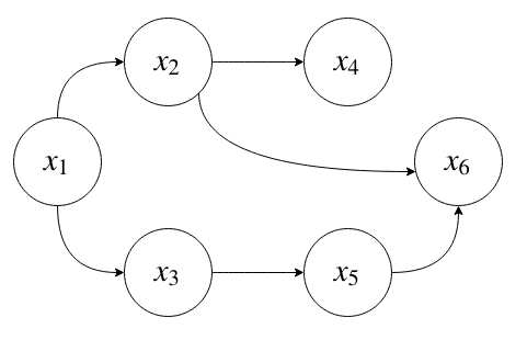
To answer the inference question, observing the state of a random variable \(X_6 = \bar x_6\), what is \(p(X_1 | \bar x_6)\)?

Note

The \(\bar x\) denotes that the variable is observed.

First, recall that the above graphical model describes a factorization of the joint distribution encoding independence between variables:

\[ p(x_1, \dots, x_6) = p(x_1) p(x_2 | x_1)p(x_3 | x_1)p(x_4 | x_2)p(x_5 | x_3)p(x_6 | x_2, x_5)\\ \]

Where the random variables under the joint distribution are inferred, observed, or marginalized respectively:

\[ \ X_F = \{x_1\}, X_E = \{x_6\}, \ X_R = \{x_2, x_3, x_4, x_5\} \]

and

\[ \begin{aligned} p(X_F | X_E) &= \frac{\sum_{X_R} p(X_F, X_E, X_R)}{\sum_{X_F, X_R} p(X_F, X_E, X_R)} \\ \Rightarrow p(x_1 | \bar x_6) &= \frac{p(x_1, \bar x_6)}{p(\bar x_6)} \\ &= \frac{p(x_1, \bar x_6)}{\sum_{x \in {X_F, X_R}}p(x, \bar x_6)} \\ \end{aligned} \]

to compute \(p(x_1, \bar x_6)\), we use variable elimination

\[ \begin{aligned} p(x_1, \bar x_6) &= p(x_1) \sum_{x_2} \sum_{x_3} \sum_{x_4} \sum_{x_5} p(x_2 | x_1)p(x_3 | x_1)p(x_4 | x_2)p(x_5 | x_3)p(\bar x_6 | x_2, x_5)\\ &= p(x_1) \sum_{x_2} p(x_2 | x_1) \sum_{x_3} p(x_3 | x_1) \sum_{x_4} p(x_4 | x_2) \sum_{x_5} p(x_5 | x_3)p(\bar x_6 | x_2, x_5) \\ &= p(x_1) \sum_{x_2} p(x_2 | x_1) \sum_{x_3} p(x_3 | x_1) \sum_{x_4} p(x_4 | x_2) p(\bar x_6 | x_2, x_3) \\ \end{aligned} \]

Note that \(p(\bar x_6 | x_2, x_3)\) does not need to participate in \(\sum_{x_4}\).

\[ \begin{aligned} &= p(x_1) \sum_{x_2} p(x_2 | x_1) \sum_{x_3} p(x_3 | x_1) p(\bar x_6 | x_2, x_3) \sum_{x_4} p(x_4 | x_2) \\ &= p(x_1) \sum_{x_2} p(x_2 | x_1) \sum_{x_3} p(x_3 | x_1) p(\bar x_6 | x_2, x_3) \\ &= p(x_1) \sum_{x_2} p(x_2 | x_1) p(\bar x_6 | x_1, x_2) \\ &= p(x_1) p(\bar x_6 | x_1) \\ \end{aligned} \]

Finally,

\[ p(x_1 \vert \bar x_6) = \frac{p(x_1) p(\bar x_6 | x_1)}{\sum_{x_1} p(x_1) p(\bar x_6 | x_1)} \]

So, we've seen that the complexity of variable elimination is related to the elimination ordering. Unfortunately, finding the best elimination ordering is NP-hard. Though, there are some heuristics.

Intermediate Factors¶

In the above examples, each time we eliminated a variable it resulted in a new conditional or marginal distribution. However, in general eliminating does not produce a valid marginal or conditional distribution of the graphical model.

Consider the distribution given by

\[ p(X,A,B,C) = p(X) p(A \vert X) p(B \vert A) p(C \vert B,X) \]

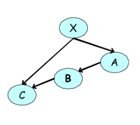
Suppose we want to marginalize over \(X\):

\[ \begin{aligned} p(A,B,C) &= \sum_X p(X) p(A \vert X) p(B \vert A) p(C \vert B,X)\\ &= p(B \vert A) \sum_X p(X) p(A \vert X) p(C \vert B,X) \end{aligned} \]

However, the resulting term \(\sum_X p(X) p(A \vert X) p(C \vert B,X)\) does not correspond to a valid conditional or marginal distribution because it is unnormalized.

For this reason we introduce factors \(\phi\) which are not necessarily normalized distributions, but which describe the local relationship between random variables.

In the above example:

\[ \begin{aligned} p(A,B,C) &= \sum_X p(X) p(A \vert X) p(B \vert A) p(C \vert B,X)\\ &= \sum_X \phi(X) \phi(A, X) \phi(A,B) \phi(X,B,C)\\ &= \phi(A,B) \sum_X \phi(X) \phi(A, X) \phi(X,B,C)\\ &= \phi(A,B) \tau(A,B,C)\\ \end{aligned} \]

In this case the original conditional distributions are represented by factors over all variables involved. This obfuscates the dependence relationship between the variables encoded by the conditional distribution. Following marginalizing over \(X\) we introduce a new factor, denoted by \(\tau\) over the remaining variables.

Note that for directed acyclic graphical models, who are defined by factorizing the joint into conditional distributions, we introduce intermediate factors to only be careful about notation.

However, there are other kinds of graphical models (e.g. undirected graphical models, and factor graphs) that are not represented by factorizing the joint into a product of conditional distributions. Instead, they factorize into a product of local factors, which will need to be normalized.

By introducing factors, even for DAGs, we can write the variable elimination algorithm for any probabilistic graphical model:

Sum-Product Inference¶

Note

The algorithm presented below is notationally verbose for generality. If you understand variable elimination algorithm presented above, this just makes the procedure precise.

Computing \(P(Y)\) for directed and undirected models is given by sum-product inference algorithm

\[ \tau(Y) = \sum_z \prod_{\phi \in \Phi} \phi(z_{Scope[\phi] \cap Z}, y_{Scope[\phi] \cap Y}) \quad \forall Y \]

where \(\Phi\) is a set of potentials or factors.

For directed models, \(\Phi\) is given by the conditional probability distributions for all variables

\[ \Phi = \{\phi_{x_i}\}^N_{i=1} = \{p(x_i | \text{parents}(x_i))\}^N_{i=1} \]

where the sum is over the set \(Z = X - X_F\). The resulting term \(\tau(Y)\) will automatically be normalized.

For undirected models, \(\Phi\) is given by the set of unnormalized potentials. Therefore, we must normalize the resulting \(\tau(Y)\) by \(\sum_Y\tau(y)\).

Example: Directed Graph¶

Take the following directed graph as example

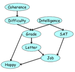
This describes a factorization of the joint distribution:

\[ p(C, D, I, G, S, L, H, J) = p(C)p(D|C)p(I)p(G | D, I)p(L | G)P(S | I)p(J | S, L)p(H | J, G) \]

And for notational convenience, we can write the conditional distributions as factors.

\[ \Phi = \{\phi(C), \phi(C, D), \phi(I), \phi(G, D, I), \phi(L, G), \phi(S, I), \phi(J, S, L), \phi(H, J, G)\} \]

If we are interested in inferring the probability of getting a job, \(P(J)\) we can perform exact inference on the joint distribution by marginalizing according to a specific variable elimination ordering.

Example: Elimination Ordering \(\prec \{C, D, I, H, G, S, L\}\)¶

\[ \begin{aligned} p(J) &=\sum_L \sum_S \phi(J,L,S) \sum_G \phi(L,G) \sum_H \phi(H,G,J) \sum_I \phi(S,I) \phi(I) \sum_D \phi(G,D,I) \underbrace{\sum_C \phi(C)\phi(C,D)}_{\tau(D)}\\ &=\sum_L \sum_S \phi(J,L,S) \sum_G \phi(L,G) \sum_H \phi(H,G,J) \sum_I \phi(S,I) \phi(I) \underbrace{\sum_D \phi(G,D,I) \tau(D)}_{\tau(G,I)}\\ &=\sum_L \sum_S \phi(J,L,S) \sum_G \phi(L,G) \sum_H \phi(H,G,J) \underbrace{\sum_I \phi(S,I) \phi(I) \tau(G,I)}_{\tau(S,G)}\\ &=\sum_L \sum_S \phi(J,L,S) \sum_G \phi(L,G) \tau(S,G) \underbrace{\sum_H \phi(H,G,J)}_{\tau(G,J)}\\ &=\sum_L \sum_S \phi(J,L,S) \underbrace{\sum_G \phi(L,G) \tau(S,G) \tau(G,J)}_{\tau(J,L,S)}\\ &=\sum_L \underbrace{\sum_S \phi(J,L,S) \tau(J,L,S)}_{\tau(J,L)}\\ &= \underbrace{\sum_L\tau(J,L)}_{\tau(J)}\\ &=\tau(J)\\ \end{aligned} \]

Note again that because our original factors correspond to marginal and conditional distributions we do not need to renormalize the final factor \(\tau(J)\). However, if we started with potential factors not from a conditional distribution, we would have to normalize \(\frac{\tau(J)}{\sum_J \tau(J)}\).

Complexity of Variable Elimination Ordering¶

We discussed previously that variable elimination ordering determines the computational complexity. This is due to how many variables appear inside each sum. Different elimination orderings will involve different number of variables appearing inside each sum.

The complexity of the VE algorithm is

\[O(m k^{N_\text{max}})\]

where

\(m\) is the number of initial factors.
\(k\) is the number of states each random variable takes (assumed to be equal here).
\(N_i\) is the number of random variables inside each sum \(\sum_i\).
\(N_\text{max} = \argmax_i N_i\) is the number of random variables inside the largest sum.

Example: Complexity of Elimination Ordering \(\prec \{C, D, I, H, G, S, L\}\)¶

Let us determine the complexity for the example above.

Here are all the initial factors:

\[ \Phi = \{\phi(C), \phi(C, D), \phi(I), \phi(G, D, I), \phi(L, G), \phi(S, I), \phi(J, S, L), \phi(H, J, G)\} \]

So \(m = \vert \Phi \vert = 8\)

Here are all the sums, and the number of random variables that appear in them

\[ \begin{aligned} &\underbrace{\sum_C \phi(C)\phi(C,D)}_{N_C = 2}\\ &\underbrace{\sum_D \phi(G,D,I) \tau(D)}_{N_D = 3}\\ &\underbrace{\sum_I \phi(S,I) \phi(I) \tau(G,I)}_{N_I = 3}\\ &\underbrace{\sum_H \phi(H,G,J)}_{N_H = 3}\\ &\underbrace{\sum_G \phi(L,G) \tau(S,G) \tau(G,J)}_{N_G = 4}\\ &\underbrace{\sum_S \phi(J,L,S) \tau(J,L,S)}_{N_S = 3}\\ & \underbrace{\sum_L\tau(J,L)}_{N_L = 2}\\ \end{aligned} \]

Therefore the largest sum is \(N_G = 4\)

For simplicity, we assume all variables take on \(k\) states.

So the complexity of the variable elimination under this ordering is \(O(8*k^4)\).

(Tutorial) Example: Elimination Ordering \(\prec \{G, I, S, L, H, C, D\}\)¶

\[ \begin{aligned} p(J) &= \sum_D \sum_C \phi(C)\phi(C,D) \sum_H \sum_L \sum_S \phi(J,L,S)\sum_I \phi(S,I)\phi(I) \underbrace{\sum_G\phi(G,D,I)\phi(L,G) \phi(H,G,J)}_{\tau(D,I,L,H,J), N_G = 6}\\ &= \sum_D \sum_C \phi(C)\phi(C,D) \sum_H \sum_L \sum_S \phi(J,L,S)\underbrace{\sum_I \phi(S,I)\phi(I) \tau(D,I,L,H,J)}_{\tau(D,L,H,J,S), N_I = 6}\\ &= \sum_D \sum_C \phi(C)\phi(C,D) \sum_H \sum_L \underbrace{\sum_S \phi(J,L,S)\tau(D,L,H,J,S)}_{\tau(D,L,H,J), N_S = 5}\\ &= \sum_D \sum_C \phi(C)\phi(C,D) \sum_H \underbrace{\sum_L \tau(D,L,H,J)}_{\tau(D,H,J), N_L = 4}\\ &= \sum_D \sum_C \phi(C)\phi(C,D) \underbrace{\sum_H \tau(D,H,J)}_{\tau(D,J), N_H = 3}\\ &= \sum_D \tau(D,J) \underbrace{\sum_C \phi(C)\phi(C,D)}_{\tau(D), N_C = 2}\\ &= \underbrace{\sum_D\tau(D,J) \tau(D)}_{\tau(J), N_D = 2}\\ &=\tau(J) \end{aligned} \]

This is a variable elimination ordering over \(m=8\) factors each with \(k\) states. The sum with the largest number of variables participating has \(N_\text{max} = 6\) so the complexity is

\[O(8 * k^6)\]

(Tutorial) Example: Elimination Ordering \(\prec \{D,C,H,L,S,I,G \}\)¶

\[ \begin{aligned} p(J) &=\sum_G \sum_I \phi(I) \sum_S \phi(S,I)\sum_L \phi(L,G) \phi(J,L,S) \sum_H \phi(H,G,J) \sum_C \phi(C)\underbrace{\sum_D \phi(G,D,I) \phi(C,D)}_{\tau(G,I,C), N_D= 4}\\ &=\sum_G \sum_I \phi(I) \sum_S \phi(S,I)\sum_L \phi(L,G) \phi(J,L,S) \sum_H \phi(H,G,J)\underbrace{\sum_C \phi(C)\tau(G,I,C)}_{\tau(G,I), N_C = 3}\\ &=\sum_G \sum_I \phi(I) \tau(G,I) \sum_S \phi(S,I)\sum_L \phi(L,G) \phi(J,L,S) \underbrace{\sum_H \phi(H,G,J) }_{\tau(G,J), N_H = 3}\\ &=\sum_G \tau(G,J) \sum_I \phi(I) \tau(G,I) \sum_S \phi(S,I)\underbrace{\sum_L \phi(L,G) \phi(J,L,S) }_{\tau(G,J,S), N_L = 4}\\ &=\sum_G \tau(G,J) \sum_I \phi(I) \tau(G,I) \underbrace{\sum_S \phi(S,I)\tau(G,J,S)}_{\tau(I,G,J), N_S = 4}\\ &=\sum_G \tau(G,J) \underbrace{\sum_I \phi(I) \tau(G,I) \tau(I,G,J)}_{\tau(G,J), N_I = 3}\\ &=\underbrace{\sum_G \tau(G,J) \tau(G,J)}_{\tau(J), N_G = 2}\\ &=\tau(J) \end{aligned} \]

This is a variable elimination ordering over \(m=8\) factors each with \(k\) states. The sum with the largest number of variables participating has \(N_\text{max} = 4\) so the complexity is

\[O(8 * k^4)\]