Message passing, Hidden Markov Models, and Sampling
This week will cover:
- Exact inference in tree-structured graphs, also known as message passing.
- An example applied to Hidden Markov Models
- How to sample from directed graphical models, called ancestral sampling.
- The basics of estimating averages by averaging samples, called Simple Monte Carlo.
Suggested reading:
- Murphy: Chapter 18
Variable Elimination Order and Trees
We learned last week that we can do exact inference by variable elimination: I.e. to compute \(P(A| C)\), we can marginalize \(P(A, B| C)\) over every variable in \(B\), one at a time.
What determines the computational time cost of variable elimination is the graph structure, and the elimination ordering. Determining the optimal elimination ordering is itself NP-complete, so unless \(P = NP\), we won't in general be able to find the optimal elimination order in a reasonable time. Even if we do, the resulting marginalization might also be unreasonably costly - remember that the time cost of marginalization is at least exponential in the number of nodes in the largest factor, and that of computing conditional distributions is #P-complete.
Heuristics for Choosing an Elimination Ordering
We won't cover these in this course, but for the curious, here are a few heuristics for estimating the cost of a given elimination ordering for a given graph:
- Min-fill: the cost of a vertex is the number of edges that need to be added to the graph due to its elimination.
- Weighted-Min-Fill: the cost of a vertex is the sum of weights of the edges that need to be added to the graph due to its elimination. Weight of an edge is the product of weights of its constituent vertices.
- Min-neighbors: the cost of a vertex is the number of neighbors it has in the current graph.
- Min-weight: the cost of a vertex is the product of weights (domain cardinality) of its neighbors.
Inference in Trees
Fortunately, there exists a general family of graphs for which the optimal elimination ordering is trivial to find, and which has only linear cost in the number of nodes! That is tree-structured graphs. Any elimination ordering that goes from the leaves inwards towards any root will be optimal. You can think of trees as just chains which sometimes branch.
Message Passing, a.k.a. computing all marginals
Belief Propagation
What if we want to compute the marginal of every variable in a graph: \(p(x_i) \ \forall x_i \in X\)?
For example, given a family tree, and the knowledge that some relatives had a certain genetic disease, we might want to compute the probability that each other person in the family tree has that disease.
We could run variable elimination separately for each variable \(x_i\), but this is more computationally expensive than it needs to be. Can we re-use the intermediate quantities?
Consider a tree:
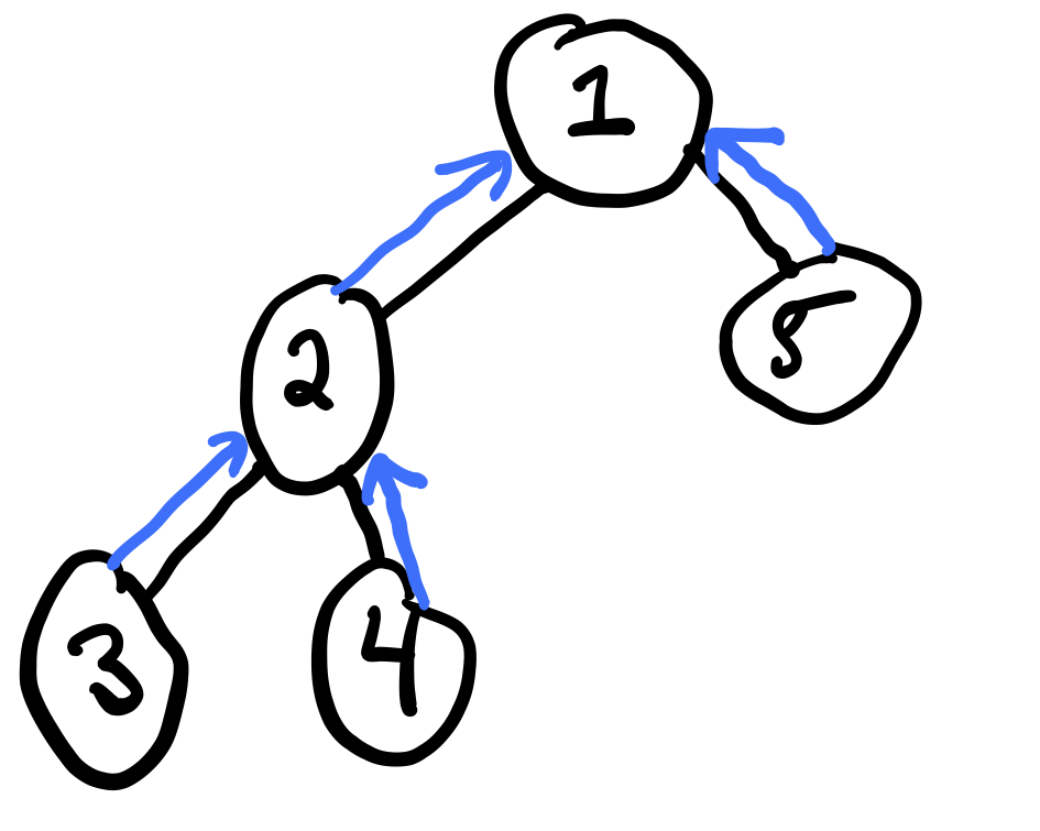
We can compute the sum product belief propagation in order to compute all marginals with just two passes. Belief propagation is based on message-passing of "messages" between neighboring vertices of the graph.
The message sent from variable \(j\) to \(i \in N(j)\) is
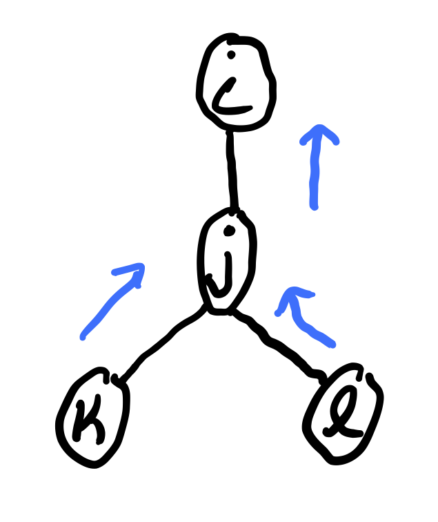
where each message \(m_{j \rightarrow i}(x_i)\) is a vector with one value for each state of \(x_i\). In order to compute \(m_j \rightarrow m_i\), we must have already computed \(m_k \rightarrow j(x_j)\) for \(k \in \mathcal N(j) \not = i\). Therefore, we need a specific ordering of the messages.
Example
Suppose we want to compute \(p(x_1)\) on the graph given above. Choosing an ordering is equivalent to choosing a root. Lets choose \(x_1\) to be the root. Then
and finally,
so
where
Elimination algorithm in trees is equivalent to message passing.
Belief Propagation Algorithm
- Choose root \(r\) arbitrarily
- Pass messages from leafs to \(r\)
- Pass messages from \(r\) to leafs
- Compute
Note that the messages coming back down the tree from the root each only depend on the information from the other branches. There is no double-counting of information.
If you try to run this algorithm on a DAG with loops (not a tree), then this is called Loopy Belief Propagation, and it gives the wrong answer in general due to this double-counting. Kind of like when someone starts a rumour and then hears the same rumour from someone else, making them more certain it's true.
Hidden Markov Models
Overview
- Markov Chains
- Hidden Markov Models
- Forward / Backward Algorithm
Sequential data
Let us turn our attention to sequential data
Broadly speaking, sequential data can be time-series (e.g. stock prices, speech, video analysis) or ordered (e.g. textual data, gene sequences). So far, we have assumed our data to be i.i.d, however this is a poor assumption for sequential data, as there is often clear dependencies between data points.
Recall the general joint factorization via the chain rule
But this quickly becomes intractable for high-dimensional data - each factor requires exponentially many parameters to specify as a function of T. So we make the simplifying assumption that our data can be modeled as a first-order Markov chain
Tip
In plain english: each observation is assumed to be independent of all previous observations except most recent.
This assumption greatly simplifies the factors in the joint distribution
A useful distinction to make at this point is between stationary and non-stationary distributions that generate our data
- Stationary Markov chain: the distribution generating the data does not change through time
- Non-stationary Markov chain: the distribution generating the data is a function of time
We are only going to consider the case of a stationary Markov chain, sometimes called a homogenous Markov chain. This means that:
meaning the process generating the data is independent of \(t\). In general you can always convert a non-stationary chain into a stationary one by appending time to the state.
Higher-order Markov chains
The first-order assumption is still very restrictive. There are many examples where this would be a poor modeling choice (such as when modeling natural language, where long-term dependencies occur often). We can generalize to high-order dependence trivially
second-order
\(m\)-order
Parameterization
How does the order of temporal dependence affect the number of parameters in our model?
Assume \(x\) is a discrete random variable with \(k\) states. How many parameters are needed to parameterize
- \(x_t\): \(k-1\), as the last state is implicit.
- first-order chain: \(k(k-1)\), as we need \(k\) number of parameters for each parameter of \(x_t\)
- \(m\)-order chain: \(k^m(k-1)\), as we need \(k^m\) number of parameters for each parameter of \(x_t\)
Aside
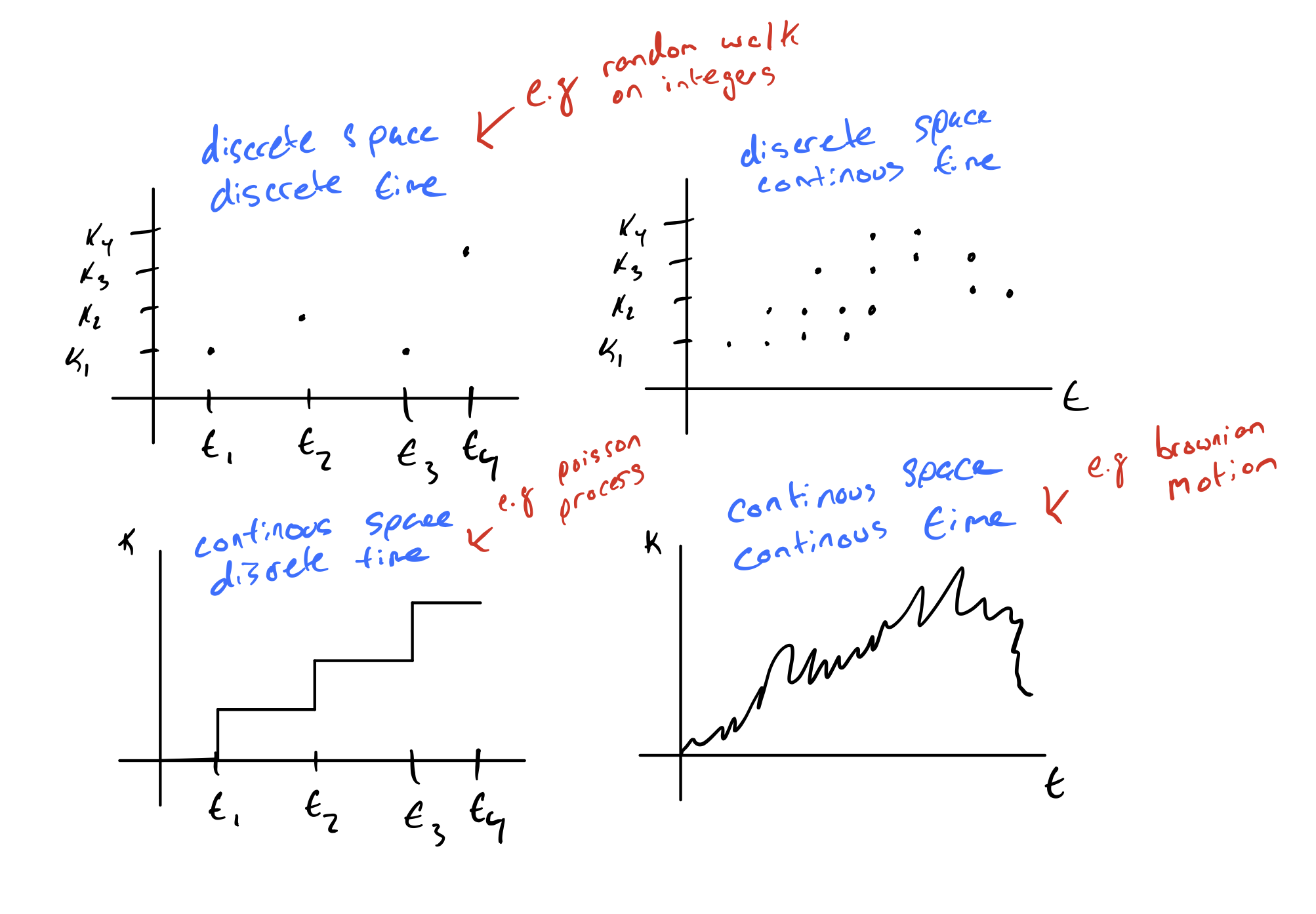
So far, we have been thinking about models that operate in discrete space and discrete time but we could also think about models that operate in continuous space or continuous time.
Hidden Markov Models
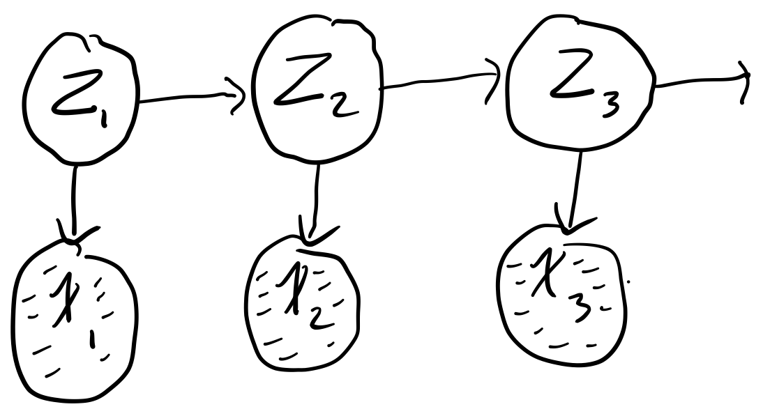
What if we want to model the fact that we don't directly observe the hidden states? For this, we introduce Hidden Markov Models (HMMs). HMMs hide the temporal dependence by keeping it in the unobserved state. For each observation \(x_t\), we associate a corresponding unobserved hidden/latent variable \(z_t\)
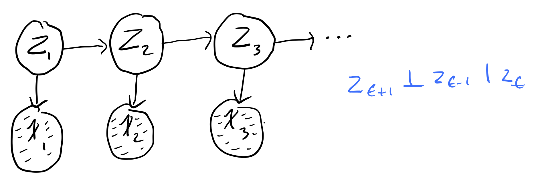
The joint distribution of the model becomes
Unlike simple Markov chains, the observations are not limited by a Markov assumption of any order. I.e. \(x_t\) isn't neceessarily independent of any other observation, no matter how many other observations we make.
Parameterizing a Hidden Markov Model
Assuming we have a homogeneous model, we only have to learn three distributions
- Initial distribution: \(\pi(i) = p(z_1 = i)\). The probability of the first hidden variable being in state \(i\) (often denoted \(\pi\))
- Transition distribution: \(T(i, j) = p(z_{t + 1} = j | z_t = i) \quad i \in \{1, ..., k\}\). The probability of moving from hidden state \(i\) to hidden state \(j\).
- Emission probability: \(\varepsilon_i(x) = p(x | z_t = i)\). The probability of an observed random variable \(x\) given the state of the hidden variable that "emitted" it.
Simple Example
Say we have the following simple chain
where
- \(x_t \in [N, Z, A]\)
- \(z_t \in [H, S]\)
where our observed states are whether or not we are watching Netflix (\(N\)), sleeping (\(Z\)), or working on the assignment (\(A\)) and our hidden states are whether we are happy (\(H\)) or sad \((S)\). Say futher that we are given the initial (\(\pi\)), transition (\(T\)), and emission probabilities (\(\varepsilon\))
| \(\pi\) | |
|---|---|
| H | 0.70 |
| S | 0.30 |
| \(\varepsilon\) | N | Z | A |
|---|---|---|---|
| H | 0.40 | 0.50 | 0.10 |
| S | 0.10 | 0.30 | 0.60 |
| T | H | S |
|---|---|---|
| H | 0.80 | 0.20 |
| S | 0.10 | 0.90 |
Note
It is the rows of these tables that need to sum to 1, not the columns!
From these conditional probabilities, we can preform inference with the model, e.g.
or
Inference in HMMs
HMMs are just tree-structured DAGs, meaning that inference in them is always cheap (in fact linear) in the number of time steps. We can use standard variable elimination and message passing to do exact inference in them. Confusingly, because they're one of the most common DAGs, there is a special name for the almost every possible inference query in them.
The main tasks we perform with HMMs are as follows:
1. Compute the probability of a latent sequence given an observation sequence
For example, computing \(p(z_{i} | x_{1:t}) \quad \forall i\). This is achieved with the Forward-Backward algorithm, which is just regular message passing.
2. Compute the marginal likelihood \(p(x_1, x_2, \dots, x_T)\) in order to fit parameters
The parameters of a HMM are sometimes learned with the Baum-Welch algorithm, a special case of the Expectation–maximization algorithm algorithm.
2. Infer the most likely sequence of hidden states
That is, we want to be able to compute \(Z^{\star} = \underset{z_{1:T}}{\operatorname{argmax}} p(z_{1:T} | x_{1:T})\). This is achieved using the Viterbi algorithm.
In this course, we will focus on the first two tasks.
Forward-backward algorithm
The Forward-backward algorithm is used to efficiently estimate the latent sequence given an observation sequence under a HMM. That is, we want to compute
assuming that we know the initial \(p(z_1)\), transition \(p(z_t | z_{t-1})\), and emission \(p(x_t | z_t)\) probabilities \(\forall_t \in [1 ,T]\). This task of hidden state inference breaks down into the following:
- Filtering: compute posterior over current hidden state, \(p(z_t | x_{1:t})\).
- Prediction: compute posterior over future hidden state, \(p(z_{t+k} | x_{1:t})\).
- Smoothing: compute posterior over past hidden state, \(p(z_n | x_{1:t}) \quad 1 \lt n \lt t\).
Our probabilities of interest, \(p(z_{t} | x_{1:T}) \quad \forall t\) are computed in two parts that are then multiplied together
- Forward Filtering: Computes \(p(z_{t} | x_{1:t}) \quad \forall \quad t\)
- Backward Filtering: Computes \(p(x_{1 + t : T} | z_t) \quad \forall \quad t\)
We note that
Note
The third line is arrived at by noting the conditional independence \(x_{t+1:T} \bot x_{1:t} | z\). If it is not clear why this conditional independence holds, try to draw out the HMM conditioned on \(z_t\).
Forward Filtering
Notice that our forward recursion contains our emission, \(p(x_t | z_t)\) and transition, \(p(z_t | z_{t-1})\) probabilities. If we recurse all the way down to \(\alpha_1(z_1)\), we get
the initial probability times the emission probability of the first observed state, as expected.
Each step has time cost \(O(K^2)\).
Backward Filtering
Notice that our backward recursion contains our emission, \(p(x_{t+1} | z_{t+1})\) and transition, \(p(z_{t+1} | z_t)\) probabilities. If we recurse all the way down to \(\beta_1(z_1)\), we get
Sampling
We will use the word "sample" in the following sense: a sample from a distribution \(p(x)\) is a single realization \(x\) whose probability distribution is \(p(x)\). This contrasts with the alternative usage in statistics, where sample refers to a collection of realizations \({x}\).
The problems to be solved
Monte Carlo methods are computational techniques that make use of random numbers. The aims of Monte Carlo methods are to solve one or both of the following problems.
Problem 1: To generate samples \(\{x^{(r)}\}^R_{r=1}\) from a given probability distribution \(p(x)\).
Problem 2: To estimate expectations of functions, \(f(x)\), under this distribution, \(p(x)\)
We will concentrate on the first problem (sampling), because if we have solved it, then we can solve the second problem by using the random samples \(\{x^{(r)}\}^R_{r=1}\) to give an estimator.
Ancestral Sampling
Given a DAG, and the ability to sample from each of its factors given its parents, we can sample from the joint distribution over all the nodes by ancestral sampling, which simply means sampling in a topoplogical order. I.e. at each step, sample from any conditional distribution that you haven't visited yet, whose parents have all been sampled. This procedure will always start with the nodes that have no parents.
Example: In a chain or HMM, you would always start with \(z_1\) and move to the right. In a tree, you would always start from the root.
Generating marginal samples
If you are only interested in sampling a particular set of nodes, you can simply sample from all the nodes jointly, then ignore the nodes you don't need.
Generating conditional samples
If you want to sample conditional on a node with no parents, that's also easy - you can simple do ancestral sampling starting from the nodes you have.
However, to sample from a DAG conditional on leaf nodes is hard in the same way that inference is hard in general. E.g. sampling the unknown key in a cryptosystem given the cyphertext but not knowing the plaintext. Finding ways to do this approximately is what a lot of the rest of the course will be about.
Simple Monte Carlo
This brings us to simple Monte Carlo:
def. Simple Monte Carlo: Given \(\{x^{(r)}\}^R_{r=1} \sim p(x)\) we estimate the expectation \(\underset{x \sim p(x)}{\operatorname{\mathbb E}} [f(x)]\) to be the estimator \(\hat \Phi\)
Properties of MC
If the vectors \(\{x^{(r)}\}^R_{r=1}\) are generated from \(p(x)\) then the expectation of \(\hat E\) is \(E\). E.g. \(\hat E\) is an unbiased estimator of \(E\).
Proof
As the number of samples of \(R\) increases, the variance of \(\hat E\) will decrease proportional to \(\frac{1}{R}\)
Proof
The accuracy of the Monte Carlo estimate depends only on the variance of \(f\), not on the dimension of \(x\). So regardless of the dimensionality of \(x\), it may be that as few as a dozen independent samples \(\{x^{(r)}\}\) suffice to estimate \(E\) satisfactorily. This is in contrast to exhaustively enumerating all possible \(x\), which has time cost exponential in the dimension of \(x\).