Stochastic Variational Inference
Suggested reading
- Murphy: Chapter 18
Overview
- Introduce TrueSkill model as an example problem.
- Review Variational Inference
- Derive the variational objective
- ELBO intuition
- Stochastic optimization
The TrueSkill latent variable model
The model we'll be examining is the TrueSkill model, a player ranking system for competitive games originally developed for Halo 2. It is a generalization of the Elo rating system in Chess. For the curious, the original paper introducing the trueskill paper can be found here: The next assignment will be based on doing variational inference in this model.
The problem that this model is supposed to solve is inferring the skill of a set of players in a competitive game, based only on observing who beats who when they play against each other. In the TrueSkill model, each player has a fixed level of skill, denoted \(z_i\). We initially don't know anything about anyone's skill, but for simplicity we'll assume everyone skill is independent. Perhaps we start with an independent Gaussian prior.
We never get to observe the players' skills directly, which makes this a latent variable model. Instead, we observe the outcome of a series of matches between different players. For each game, the probability that player \(i\) beats player \(j\) is given by \(\sigma(z_i - z_j)\) where sigma is the logistic function: \(\sigma(y) = \frac{1}{1 + \exp(-y)}\). So we can write:
The exact form of the prior and likelihood aren't particularly important, as long as the win probability for player 1 is nondecreasing in \(z_i\) and nonincreasing for \(z_j\). So the higher the skill level, the higher the chance of winning each game.
We can write the entire joint likelihood of a set of players and games as:
Let's draw the prior, likelihood, and posterior for two players. What happens if we see two players both beat each other? Is that different than not seeing any matches at all?
It's hard to draw a graphical model for this joint distribution, but we can draw the graphical model for 3 players that have two games between them, and see that given the outcome of some matches, the players' skills are no longer independent, even if they've never played each other.
Computing even the posterior over two players' skills requires integrating over all the other players' skills:
Posterior Inference in Latent Variable Models
Consider the probabilistic model \(p(x, z)\) where
- \(x_{1:T}\) are the observations
- \(z_{1:N}\) are the unobserved latent variables
The conditional distribution of the unobserved variables given the observed variables (the posterior inference) is
which we will denote as \(p_{\theta}(z | x)\).
Whenever the number of values that \(z\) can take is largte, the computation (\int p(x, z)d_z) is intractable, making the computation of the conditional distribution itself intractable. Thus we have to use approximate inference. In today's lecture, we'll learn about variational inference.
Approximating the Posterior Inference with Variational Methods
Approximation of the posterior inference with variational methods works as follows:
- Introduce a variational family \(q_\phi(z)\) with parameters \(\phi\).
- Encode some notion of "distance" between \(p(z | x)\) and \(q_\phi(z)\).
- Minimize this distance.
This turns Bayesian Inference into an optimization problem, and if enough parts of our model are differentiable and well-approximated by simple Monte Carlo, we can use stochastic gradient descent to solve this optimization problem scalably.
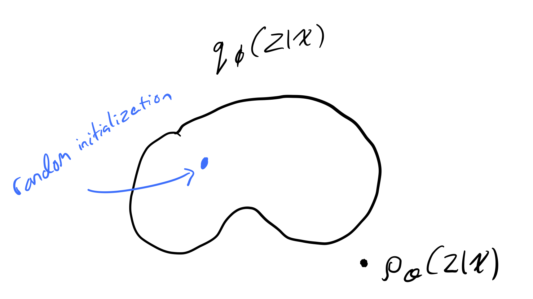
Note that whatever parametric family of functions we choose for \(q_\phi(z)\), it is unlikely that this variational family will have the true posterior \(p(z|x)\) in it.
The earliest versions of variational inference optimized directly in function space, and required the calculus of variations, but now we use a simpler method that only requires standard finite-dimensional calculus.
Show autograd demo:
Answering questions with an approximate posterior:
Once we have this approximate posterior, what can we do with it?
We can find approximate answers to questions about the true posterior. For example: in the Trueskill example, the sorts of questions we might want to answer are:
- Is player A better than player B?
- What is the player with closest skill to B? (for matchmaking)
We can express question as an expectation:
which we could easily approximate with simple Monte Carlo if we could sample from \(p(z_A, z_B | x)\). However, we can't. But if we had a good approximate posterior, we could! For example, we could sample from \(q(z|x)\).
We could answer question two by simply examining the mean of \(q(z_i | x)\) for each \(i\), or estimate it by simple Monte Carlo if it's not available in closed form.
Kullback-Leibler Divergence
We will measure the distance between \(q_\phi\) and \(p\) using the Kullback-Leibler divergence.
Note
Kullback–Leibler divergence has lots of names, we will stick to "KL divergence".
We compute \(D_{KL}\) as follows:
Properties of the KL Divergence
- \(D_{KL}(q_\phi || p) \ge 0\)
- \(D_{KL}(q_\phi || p) = 0 \Leftrightarrow q_\phi = p\)
- \(D_{KL}(q_\phi || p) \not = D_{KL}(p || q_\phi)\)
The significance of the last property is that \(D_{KL}\) is not a true distance measure.
Variational Objective
We want to approximate \(p\) by finding a \(q_\phi\) such that
but the computation of \(D_{KL}(q_\phi || p)\) is intractable (as discussed above).
Note
\(D_{KL}(q_\phi || p)\) is intractable because it contains the term \(p(z | x)\), which we have already established, is intractable.
To circumvent this issue of intractability, we will derive the evidence lower bound (ELBO), and show that maximizing the ELBO \(\Rightarrow\) minimizing \(D_{KL}(q_\phi || p)\).
Where \(\mathcal L(\phi ; x)\) is the ELBO.
Note
Notice that \(\log p(x)\) is not dependent on \(z\).
Rearranging, we get
Because \(D_{KL}(q_\phi (z | x) || p (z | x)) \ge 0\)
\(\therefore\) maximizing the ELBO \(\Rightarrow\) minimizing \(D_{KL}(q_\phi (z | x) || p (z | x))\).
Optimizing the ELBO
We have that
If we want to optimize this with gradient methods, we will need to compute \(\nabla_\phi \mathcal L(\phi)\):
we know from a previous lecture that one can get an unbiased estimator of any expectation as long as we can sample from the distribution and evaluate the function, using simple Monte Carlo.
Pathwise Gradient
Here, we have the gradient of an expectation. Let's turn it into an expectation by switching the derivative and expectation operators. However, in general, we can't switch the derivative and the expectation if the distribution we're taking the expectation over depends on the parameter. So let's factor out the randomness from \(q\), and put it unto a parameterless, fixed source of noise \(p(\epsilon)\). To do this, we need to find a function \(T(\epsilon, \phi)\) such that if:
Usually we start with \(p(\epsilon)\) being uniform or Normal. It's not always easy to find these functions here's a list, and we already know one for transforming standard normals into Gaussians with a given mean and variance:
Using this trick, we can write our expectation, and then move the gradient inside:
And that's it! Now we have a differentiable function that we can estimate with simple Monte Carlo. Additionally, if \(p(x|z)\) factorizes over the points in the dataset, we can speed up computation by randomly subsampling the data at each iteration as well. These two tricks together mean that SVI can be used to fit models with millions of parameters on millions of datapoints.
We simply need to code up \(T(\epsilson, \phi), \log p(x|z), \log p(z)\) and \( \log q_\phi(z|x))\) in a language or package that supports automatic differentiation, and we will get the gradient for free.
There are some notable extensions we'll cover or mention in this course: 1. We can make \(q_\phi\) arbitrarily expressive, for instance using a mixture of Gaussians, or a normalizing flow. 2. We can fit both \(\phi\) and parameters of \(p(z|x)\) at the same time. For instance, we might want to learn the shape of the function that determines the probability of a win given both players' skills.
Appendix
Extra Demos:
Bayesian neural network demo: or youtube video of demo
Useful Resources
- High level overview on variational inference.
Tutorial
Alternative Derivation
Starting with Jenson's inequality,
if \(X\) is a random variable and \(f\) is a convex function.
Given that \(\log\) is a concave function, we have
Alternative Forms of ELBO and Intuitions
We have that
1) The most general interpretation of the ELBO is given by
2) We can also re-write 1) using entropy
3) Another re-write and we arrive at
This frames the ELBO as a tradeoff. The first term can be thought of as a "reconstruction likelihood", i.e. how probable is \(x\) given \(z\), which encourages the model to choose the distribution which best reconstructs the data. The second term acts as regularization, by enforcing the idea that our parameterization shouldn't move us too far from the true distribution.
Mean Field Variational Inference
In mean field variational inference, we restrict ourselves to variational families \(q\) that full factorizes to \(q_\phi(z)\) (no \(x\)!). I.e., we approximate \(p(z|x)\) with \(q_\phi(z)\)
Traditional Variational Inference (ASIDE)
If \(q\)s are in the same family as \(p\)s, we can optimize via coordinate ascent.
- Fix all other variables → optimize local
- Aggregate local → optimize global
- Repeat until KL divergence
Score function Gradient etimator
Also called the likelihood ratio, or REINFORCE, was independently developed in 1990, 1992, 2013, and 2014 (twice). It is given by
if we assume that \(q_\phi(z)\) is a continous function of \(\phi\), then
using the log-derivative trick \(\big ( \nabla_\phi \log q_\phi = \frac{\nabla_\phi q_\phi}{q_\phi} \big )\):
where \(q_\phi(z | x )\) is the score function. Finally, we have
which is unbiased, just like the pathwise gradient, but usually much higher variance. One of the main reasons variational inference wasn't used much until recently was that it wasn't widely understood how big the improvement in variance is in high dimensions.