Directed Graphical Models
Suggested Reading
- Murphy: Chapters 10-12 (excluding * sections)
- Kevin Murphy's page on graphical models
Overview
- Decision theory
- Graphical notation
- Conditional independence
- Bayes Ball
- Latent variables
- Common motifs
Decision Theory
Why do we care about probabilities in the first place? Answer: They help us make decisions.
Pascal, 1670: When faced with a choice of actions, you should:
- Determine the value of all possible outcomes.
- Find the probability of each outcome under each action.
- Multiply the two to get expected value, summing over all outcomes.
- Choose the action with highest expected value.
Example:
I think I might have a bacterial infection. Should I 1. Do nothing, 2. Take penicillin, 3. Take more effective but toxic last-line antibiotics?
First, we list possible outcomes and their values:
| Outcome | value |
|---|---|
| No infection, no toxins. | 0 days sick |
| Infection, no toxins. | 5 days sick |
| No infection, but toxins. | 1 day sick |
| Infection and toxins. | 8 days sick |
Second, we need the probability of each outcome under each possible action:
| P(outcome given action): | Nothing | Penicillin | Last-line |
|---|---|---|---|
| No infection, no toxins. | 0.1 | 0.9 | 0 |
| Infection, no toxins. | 0.9 | 0.1 | 0 |
| No infection, toxins. | 0 | 0 | 0.99 |
| Infection and toxins. | 0 | 0 | 0.01 |
| --- | --- | --- | --- |
| Sum | 1 | 1 | 1 |
Third, for each action we compute the sum of all values times their probability, ignoring all zeros:
- Do nothing: 0.9 * 5 = 4.5 expected days sick.
- Take penicillin 0.1 * 5 = 0.5 expected days sick.
- Take toxic last-line antibiotics: 0.99 * 1 + 0.01 * 8 = 1.07 expected days sick.
Option with lowest expected number of days sick: penicillin.
Objections:
A few common objections to this framework:
Objection 1: I don't care about about the average outcome. I want to make sure my plane never crashes, or my bridge never falls.
Answer: You can't guarantee anything, you can only make probabilities small. So you have to assign values to probabilistic outcomes, and the only coherent way to do this is linearly. I.e. twice the probability = twice as bad.
Objection 2: You can't compare the pain of being sick to the cost of medicine.
Answer: We usually have to make tradeoffs, so we should be explicit about what we value so that we can discuss it. The World Health Organization estimated the relative quality people assigned to their own lives under different disabilities:
| Condition | Life discount factor |
|---|---|
| Dementia | 0.666 |
| Blindness | 0.594 |
| Schizophrenia | 0.528 |
| AIDS, not on ART | 0.505 |
| Burns 20%-60% of body | 0.441 |
| Fractured femur | 0.372 |
| Moderate depression episode | 0.350 |
| Amputation of foot | 0.300 |
| Deafness | 0.229 |
| Infertility | 0.180 |
| Amputation of finger | 0.102 |
| Lower back pain | 0.061 |
Objection 3: It's hard to compute probabilities and expectations over all possible outcomes.
Answer: I know! That's what the tools in this course will help with.
Where did P(outcome | action) come from? That's what the rest of the course is about. In general these numbers will also be expectations over joint distributions many possible variables, like which infection we have, the details of our own physiology. We can always make the model more detailed to include more information.
But this is ultimately what we're going to do with these probabilities: Use them to make informed decision to make our lives better.
Joint distributions.
The joint distribution of \(N\) random variables is a very general way to encode knowledge about a system.
In general, a discrete distribution of \(N\) variables each of which can take \(K\) states requires \(K^N - 1\) parameters to specify.
They can always be decomposed into a set of simpler conditional distributions by the chain rule of probability
this is true for any joint distribution over any random variables. For example, a application of the chain rule for two random variables gives
and for \(N\) random variables
for all possible orderings.
This decomposition doesn't reduce the number of parameters.
Conditional Independence
Two random variables \(A\), \(B\) are conditionally independent given a third variable \(C\), denoted
\[X_A \perp X_B | X_C\]
if
for all \(X_c\).
Only a subset of all joint distributions respect any given conditional independence statement.
Graphical models
Probabilistic graphical models are a concise way to specify and reason about conditional independencies, without worrying about the detailed form of the distribution. There are three flavours:
- Undirected
- Factor graphs
- Directed
This couse will focus on directed models, since they are the most commonly encountered, and are relatively interpretable.
Directed acyclic graphical models
A directed graphical model implies a restricted factorization of the joint distribution. In a DAG, variables are represented by nodes, and edges represent dependence.
As above, for any joint distribution of random variables \(x_1, x_2, \dots, x_N\), we can write:
for any ordering of the nodes.
The meaning of any particular A directed acyclic graphical model \(D\) is that
where \(\textnormal{parents}_M(x_i)\) is the set of nodes with edges pointing to \(x_i\).
In other words, the joint distribution of a DAGM factors into a product of local conditional distributions, where each node (a random variable) is conditionally dependent on its parent node(s), which could be empty.
For example, the graphical model
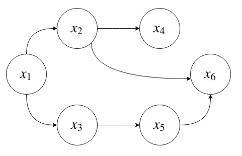
corresponds to the following factorization of the joint distribution:
Suppose each is \(x_i\) is a binary random variable. How many parameters does it take to represent this joint distribution?
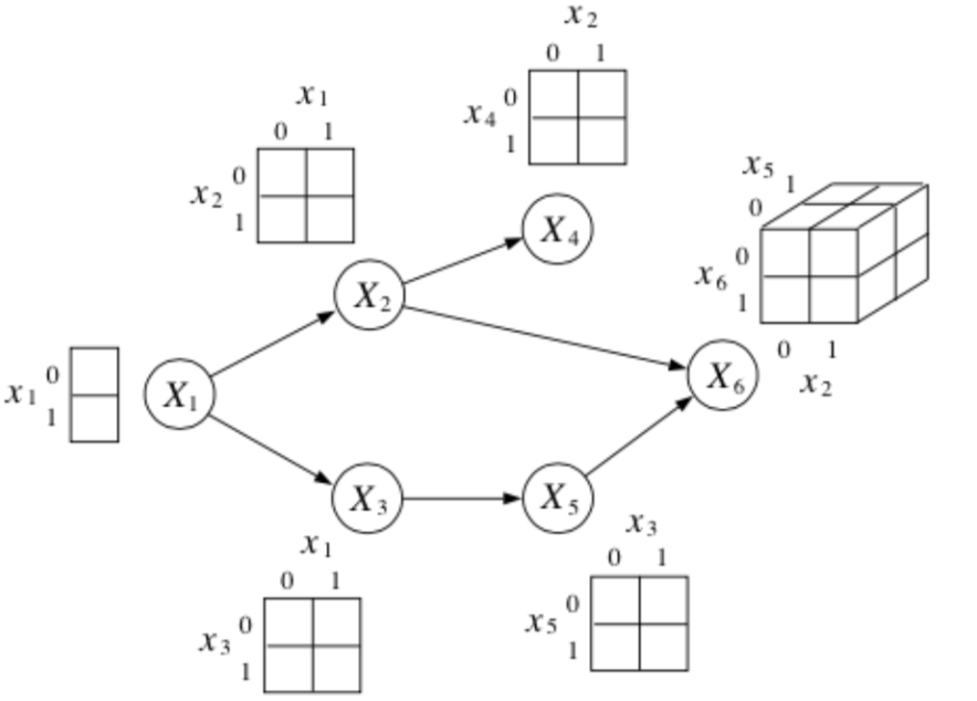
where each conditional probabilty table with \(K\) parents requires \(2^K\) parameters.
If we allow all possible conditional dependencies, that corresponds to a fully-connected DAG:
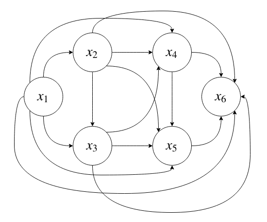
which will require \(2^N - 1\) parameters to specify.
Since we only condition on parent nodes as opposed to every node, this distribution is exponential in the fan-in of the nodes (the number of nodes in the parent set), instead of in \(N\).
In general, it's computationally infeasible to work with fully-flexible distributions like this one, both because of the computational burden, and because it's hard to fit so many parameters accurately.
We can reduce the number of parameters in a model, and also reduce the computational burden of making inferences by introducing conditional independencies. This might not be a bad approximation in some settings.
Grouping variables
We can always group variables together into one bigger variable.
as
Conditional Independence in DAGMs
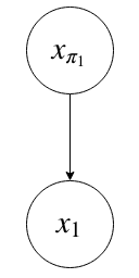
From Kevin Murphy: The simplest conditional independence relationship encoded in a Bayesian network can be stated as follows: a node is independent of its ancestors given its parents:
In general, missing edges imply conditional independence. The next part of this lecture will be about how to determine which conditional independencies hold given a DAG.
D-Separation
D-separation, or directed-separation is a notion of connectedness in DAGs in which two (sets of) variables may or may not be connected conditioned on a third (set of) variable(s). D-connection implies conditional dependence and d-separation implies conditional independence.
In particular, we say that
if every variable in \(A\) is d-separated from every variable in \(B\) conditioned on all the variables in \(C\). We will look at two methods for checking if an independence is true: A depth-first search algorithm and Bayes Balls.
DFS Algorithm for checking independence
To check if an independence is true, we can cycle through each node in \(A\), do a depth-first search to reach every node in \(B\), and examine the path between them. If all of the paths are d-separated (i.e., conditionally independent), then
It will be sufficient to consider triples of nodes. Let's go through some of the most common triples.
1. Chain
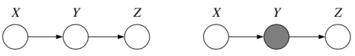
Question: When we condition on \(y\), are \(x\) and \(z\) independent?
Answer:
From the graph, we get
which implies
\(\therefore\) \(P(z | x, y) = P(z | y)\) and so by \(\star\star\), \(x \bot z | y\).
Tip
It is helpful to think about \(x\) as the past, \(y\) as the present and \(z\) as the future when working with chains such as this one.
2. Common Cause
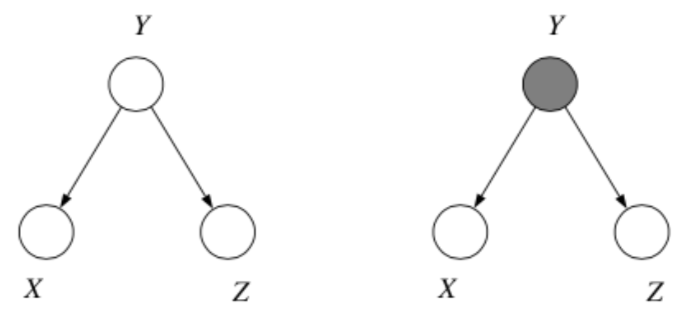
Where we think of \(y\) as the "common cause" of the two independent effects \(x\) and \(z\).
Question: When we condition on \(y\), are \(x\) and \(z\) independent?
Answer:
From the graph, we get
which implies
\(\therefore\) \(P(x, z| y) = P(x|y)P(z|y)\) and so by \(\star\), \(x \bot z | y\).
3. Explaining Away
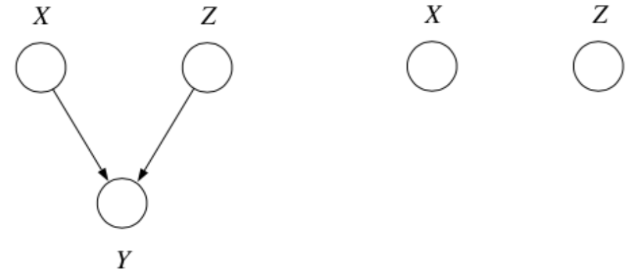
Question: When we condition on \(y\), are \(x\) and \(z\) independent?
Answer:
From the graph, we get
which implies
\(\therefore\) \(P(z | x, y) \not = P(z|y)\) and so by \(\star\star\), \(x \not \bot z | y\).
In fact, \(x\) and \(z\) are marginally independent, but given \(y\) they are conditionally dependent. This important effect is called explaining away (Berkson’s paradox).
Example
Imaging flipping two coins independently, represented by events \(x\) and \(z\). Furthermore, let \(y=1\) if the coins come up the same and \(y=0\) if they come up differently. Clearly, \(x\) and \(z\) are independent, but if I tell you \(y\), they become coupled!
Bayes-Balls Algorithm
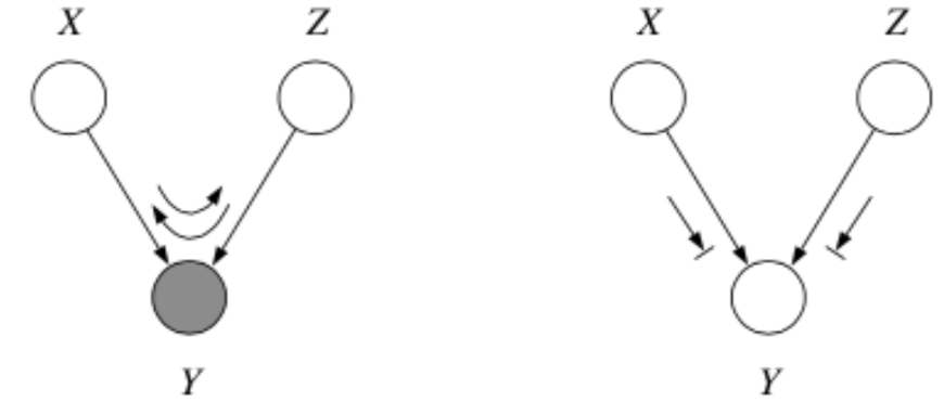
A particular algorithm for determining conditional independence in a DAGM is the Bayes Ball algorithm. To check if \(x_A \bot x_B | x_C\) we need to check if every variable in \(A\) is d-seperated from every variable in \(B\) conditioned on all variables in \(C\). In other words, given that all the nodes in \(x_C\) are "clamped", when we "wiggle" nodes \(x_A\) can we change any of the nodes in \(x_B\)?
In general, the algorithm works as follows:
- Shade all nodes \(x_C\)
- Place "balls" at each node in \(x_A\) (or \(x_B\))
- Let the "balls" "bounce" around according to some rules
- If any of the balls reach any of the nodes in \(x_B\) from \(x_A\) (or \(x_A\) from \(x_B\)) then \(x_A \not \bot x_B | x_C\)
- Otherwise \(x_A \bot x_B | x_C\)
The rules are as follows:
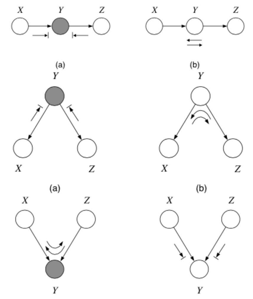
including the boundary rules:

where arrows indicate paths the balls can travel, and arrows with bars indicate paths the balls cannot travel.
Note
Notice balls can travel opposite to edge directions!
Here’s a trick for the explaining away case: If \(y\) or any of its descendants is shaded, the ball passes through.
Tip
See this video for an easy way to remember all 10 rules.
Examples
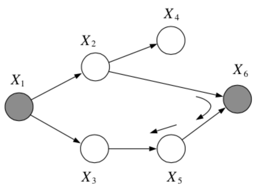
Question: In the following graph, is \(x_1 \bot x_6 | \{x_2, x_3\}\)?
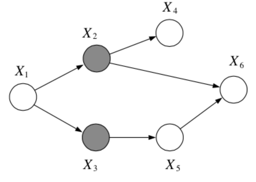
Answer:
Yes, by the Bayes Balls algorithm.
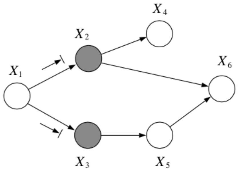
Question: In the following graph, is \(x_2 \bot x_3 | \{x_1, x_6\}\)?
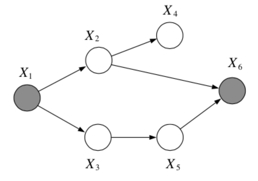
Answer:
No, by the Bayes Balls algorithm.
Example of a DAGM: Markov Chain
Markov chains are a stochastic model describing a sequence of possible events in which the probability of each event depends only on the state attained in the previous event.
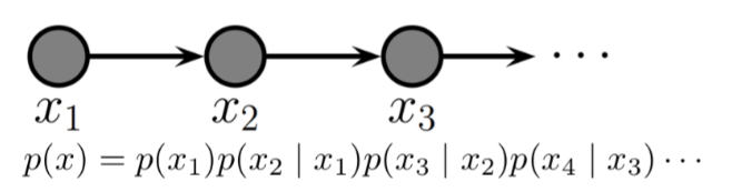
In other words, it is a model that satisfies the Markov property, i.e., conditional on the present state of the system, its future and past states are independent.
Plates
Because Bayesian methods treat parameters as random variables, we would like to include them in the graphical model. One way to do this is to repeat all the iid observations explicitly and show the parameter only once. A better way is to use plates, in which repeated quantities that are iid are put in a box
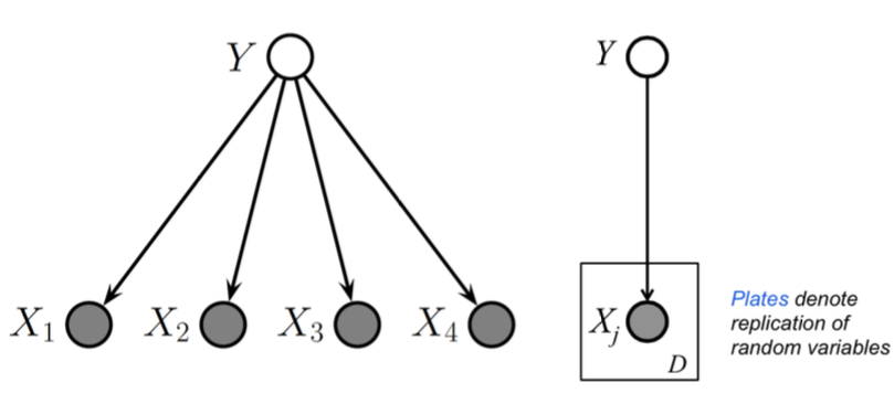
Plates are like “macros” that allow you to draw a very complicated graphical model with a simpler notation. The rules of plates are simple: repeat every structure in a box a number of times given by the integer in the corner of the box (e.g. \(N\)), updating the plate index variable (e.g. \(n\)) as you go. Duplicate every arrow going into the plate and every arrow leaving the plate by connecting the arrows to each copy of the structure.
Nested Plates
Plates can be nested, in which case their arrows get duplicated also, according to the rule: draw an arrow from every copy of the source node to every copy of the destination node.
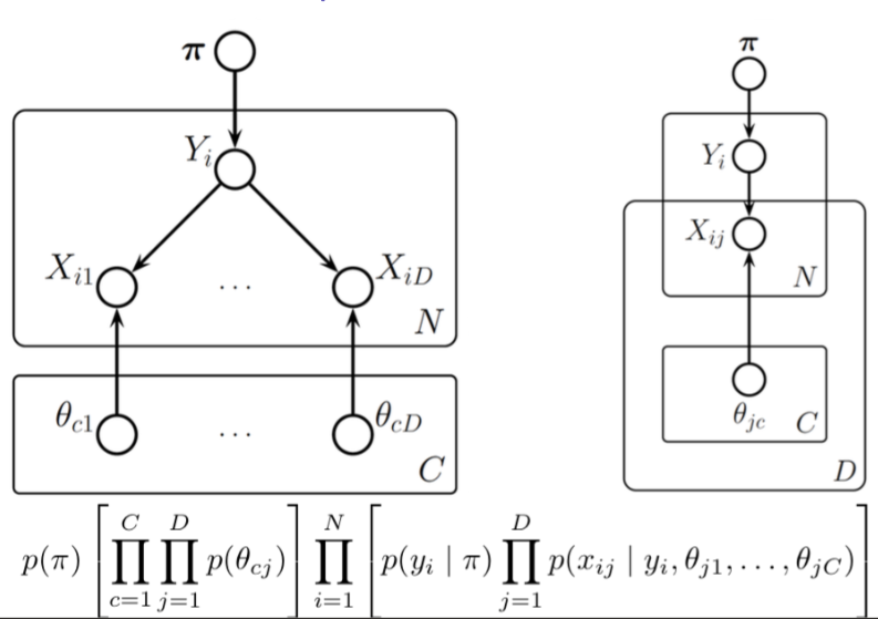
Plates can also cross (intersect), in which case the nodes at the intersection have multiple indices and get duplicated a number of times equal to the product of the duplication numbers on all the plates containing them.
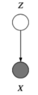
Unobserved Variables
Certain variables in our models may be unobserved (\(Q\) in the example given below), either some of the time or always, at training time or at test time.
Graphically, we use shading to indicate observation.
Partially Unobserved (Missing) Variables
If variables are occasionally unobserved then they are missing data, e.g., undefined inputs, missing class labels, erroneous target values. In this case, we can still model the joint distribution, but we marginalize the missing values:
\[\ell(\theta ; \mathcal D) = \sum_{\text{complete}} \log p(x^c, y^c | \theta) + \sum_{\text{missing}} \log p(x^m | \theta)\] \[= \sum_{\text{complete}} \log p(x^c, y^c | \theta) + \sum_{\text{missing}} \log \sum_y p(x^m, y | \theta)\]
Note
Recall that \(p(x) = \sum_q p(x, q)\).
Latent variables
What to do when a variable \(z\) is always unobserved? Depends on where it appears in our model. If we never condition on it when computing the probability of the variables we do observe, then we can just forget about it and integrate it out.
E.g., given \(y\), \(x\) fit the model \(p(z, y|x) = p(z|y)p(y|x, w)p(w)\). In other words if it is a leaf node.
However, if \(z\) is not a leaf node, marginalizing over it will induce dependencies between its children.
E.g. given \(y\), \(x\) fit the model \(p(y|x) = \sum_z p(y|x, z)p(z)\).
Where do latent variables come from?
Latent variables may appear naturally, from the structure of the problem (because something wasn’t measured, because of faulty sensors, occlusion, privacy, etc.). But we also may want to intentionally introduce latent variables to model complex dependencies between variables without specifying the dependencies between them directly.
Mixture models
What if the class is unobserved? Then we sum it out
We can use Bayes' rule to compute the posterior probability of the mixture component given some data:
these quantities are called responsibilities.
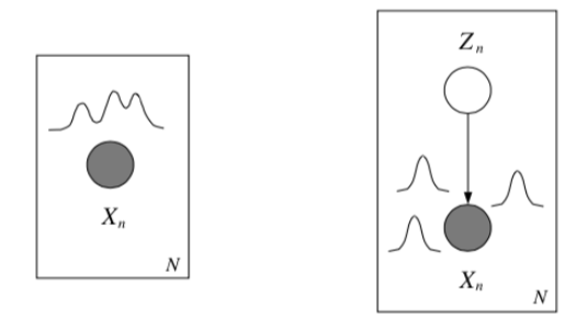
Example: Gaussian Mixture Models
Consider a mixture of \(K\) Gaussian componentns
- Density model: \(p(x | \theta)\) is the marginal density.
- Clustering: \(p(z | x, \theta)\) is cluster assignment probability.
- Fitting: \(p(z = k | x, \theta)\) is the log marginal likelihood.
Tutorial
Below are some detailed examples of the above concepts.
Second-order Markov chain
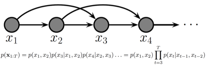
The earlier images depicts a first-order Markov chain, this is a second-order Markov chain.
Hidden Markov Models (HMMs)
Hidden Markov Model (HMM) is a statistical Markov model in which the system being modeled is assumed to be a Markov process with unobserved (i.e. hidden) states. It is a very popular type of latent variable model
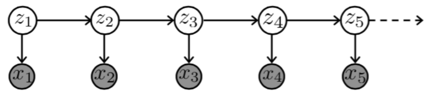
where
- \(Z_t\) are hidden states taking on one of \(K\) discrete values
- \(X_t\) are observed variables taking on values in any space
the joint probability represented by the graph factorizes according to
Conditional independence examples and Bayes Ball
Example: Explaining away from Kevin Murphy's tutorial
From Kevin Murphy's page on graphical models: Consider a college which admits students who are either brainy or sporty (or both!). Let C denote the event that someone is admitted to college, which is made true if they are either brainy (B) or sporty (S). Suppose in the general population, B and S are independent. We can model our conditional independence assumptions using a graph which is a V structure, with arrows pointing down.
Now look at a population of college students (those for which C is observed to be true). It will be found that being brainy makes you less likely to be sporty and vice versa, because either property alone is sufficient to explain the evidence on C.
Example: Mixtures of Experts
Think about the following two sets of data, and notice how there is some underlying structure not dependent on x.
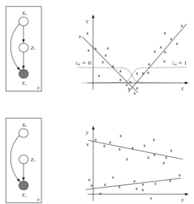
The most basic latent variable model might introduce a single discrete node, \(z\), in order to better model the data. This allows different submodels (experts) to contribute to the (conditional) density model in different parts of the space (known as a mixture of experts).
Mixtures of experts, also known as conditional mixtures are exactly like a class-conditional model, but the class is unobserved and so we sum it out:
where \(\sum_k \alpha_k (x) = 1 \; \forall x\). This is a harder problem than the previous example, as we must learn \(\alpha(x)\), often called the gating function (unless we chose \(z\) to be independent of \(x\)). However, we can still use Bayes' rule to compute the posterior probability of the mixture components given some data:
Example: Mixtures of Linear Regression Experts
In this model, each expert generates data according to a linear function of the input plus additive Gaussian noise
where the gating function can be a softmax classifier
Remember: we are not modeling the marginal density of the inputs \(x\).
Gradient learning with mixtures
We can learn mixture densities using gradient descent on the likelihood as usual.
In other words, the gradient is the responsibility weighted sum of the individual log likelihood gradients
Tip
We used two tricks here to derive the gradient, \(\frac{\partial \log f(\theta)}{\partial \theta} = \frac{1}{f(\theta)} \cdot \frac{\partial f(\theta)}{\partial \theta}\) and \( \frac{\partial f(\theta)}{\partial \theta} = f(\theta) \cdot \frac{\partial \log f(\theta)}{\partial \theta} \)
Useful Resources
- Metacademy lesson on Bayes Balls. In fact, that link will bring you to a short course on a couple important concepts for this course, including conditional probability, conditional independence, Bayesian networks and d-separation.
- A video on how to memorize the Bayes Balls rules (this is linked in the above course).