Week 11: Amortized Inference and Variational Auto Encoders
Using HMC to infer transmission + death rates for COVID: paper
External Resources
- Keras Blog on autoencoders.
- Blog on VAEs.
- Blog on the intuitive understanding of VAEs.
- The original VAE paper (which assignment 3 is based on) and a video explanation.
- Blog on the reparameterization trick.
- Paper on lower-variance gradients
Recap: latent variable models
Writing down a generative model \(p_\theta(x|z), p_\theta(z)\) is a simple, interpretable and powerful way to specify a complicated joint distribution \(p(x)\).
Examples
- Trueskill gives a joint distribution over game outcomes. Can interpret posterior over latent quantities as a belief state about skills given games.
- Personality models (e.g. Big 5 traits) (z = personality, x is behavior), aka factor analysis.
- Item Response Theory,
- Latent Growth models.
What's easy?
- Sampling \(z \sim p(z)\) and \(x \sim p(x|z)\), and \(x, z \sim p(x|z)\), \(x \sim p(x)\)
- Evaluating \(p(z)\) and \(p(x|z)\), and \(p(x|z)\), including e.g. \(p(x_1, x_2|x_3, x_4)\)
What's hard?
- Sampling \(z \sim p(z|x)\) or \(x_1, x_2 \sim p(x_1, x_2|x_3, x_4)\)
- Evaluating \(p(z|x)\) or \(p(x_1, x_2|x_3, x_4)\), \(p(x)\)
- \(p(x) = \int p(x|z)p(z) dz\) (and simple MC will have high variance)
- \(p(x_1, x_2|x_3, x_4) = \int p(x_1, x_2|z)p(z|x_3, x_4) dz \) (need posterior)
- \(p(z|x) = \frac{p(x, z)}{\int p(x, z) dz}\)
Recap: Stochastic variational inference
To approximate \(p(x|z)\): 1. Introduce a variational family \(q_\phi(z|x)\) with parameters \(\phi\). 2. Minimize KL divergence between \(p(z | x)\) and \(q_\phi(z|x)\).
Tip
Big distinction between model \(p(x,z)\) and approximate inference strategy. Can use different approx. inf. for same model (such as MCMC or loopy belief propagation), even ones that weren't invented when you wrote down the model!
This is equivalent to maximizing a lower bound on the log marginal likelihood \(\log p(x)\):
We'll want to optimize using stochastic unbiased gradients from simple Monte Carlo. We can use thereparameterization trick to bring the gradient inside the expectation:

Per-example latent variable models
In the Trueskill model, there is one big vector of \(z\)s, and one big list of game outcomes \(x\).
The graphical model for Trueskill is just one big z to one big z.
The graphical model for the approximate posterior is just z.
What about our personality quiz example? E.g. there are N people each of whom takes a quiz with D questions. And we assume each person has an a priori indepedently distributed, Q-dimensional vector that specifies their personality. Then there is a separate \(z\) vector for each \(x\) vector. The graphical model will have a plate.
The true posterior in this model factorizes over people. But now we have N true posteriors to approximate. How could we do efficient approximate inference in this setting?
Motivation #1: SVI on a per-example LVM doesn't scale to large data
This argument is a bit involved, so feel free to zone out.
We could simply do SVI on everyone's \(z\) vectors all at once on each iteration of gradient descent. Each person would have a \(\phi_i\). The graphical model would also have a plate. This is a good strategy for a small N. However, if N is large, we want to be able to subsample the data. However, in this case, we would have one global \(\theta\) and a separate approximate posterior \(q_{\phi_i}(z_i|x_i)\) for each person. If we subsampled one out of a thousand people each time we updated \(\theta\), then each \(q_{\phi_i}(z_i|x_i)\) would be a thousand steps out of date. Keep in mind that the true posterior will change shape as the model parameters \(\theta\) change. So the gradients that \(\theta\) would get will be for a very poor approximate posterior. We could stop and optimze each \(q_{\phi_i}(z_i|x_i)\) for a while before we get the gradient for \(theta\), but this would also be slow.
We want to be able to somehow keep all the approximate posteriors in sync, without optimizing all of them whenever we update \(\theta\).
Motivation #2: People can learn to recognize what's going on from partial evidence
For example, with enough experience, doctors, plumbers, detectives, etc. can very quickly tell what is going on and what they still need more information about, if they've seen enough similar situations. Perhaps we could somehow train a neural network to look at the data for a person \(x_i\), and then output an approximate posterior \(q_{\phi_i}(z_i|x_i)\)?
Amortized Inference
"Amortize" just means "spread out a cost over time". Instead of doing SVI from scratch every time we see a new datapoint, we're going to try to gradually learn a function that can look at the data for a person \(x_i\), and then output an approximate posterior \(q_\phi(z_i|x_i)\). We'll call this a "recognition model" Instead of a separate \(\phi_i\) for each data example, we'll just have a single global \(\phi\) that specifies the parameters of the recognition model. Because the relationship between data and posteriors is complex and hard to specify by hand, we'll do this with a neural network!
We've already seen one way to specify a probability distribution given an input with neural networks. We can simply have a network take in \(x_i\), and output the mean and variance vector for a Gaussian:
The graphical model for this recognition model has the \(\phi\) outside the plate.
The algorithm for amortized inference looks like: 1. Sample a datapoint 2. Compute params of approximate posterior (recognition) 3. Compute gradient of Monte Carlo estimate of ELBO wrt phi. 4. Update phi
Then, when we want to make predictions about a new datapoint, we can use our fast recognition model if we want! Of course, we might also want to stop and do something slower but more accurate, like per-example SVI, or MCMC.
Also optimizing model parameters.
If \(\log p_\theta(x)\) depends on parameters \(\theta\), then the ELBO is a function of both, and we can optimize them together:
In the trueskill example, this would let us learn the shape of the likelihood function, for example:
Thus we can jointly fit the model parameters and the recognition network, by subsampling training examples and using simple Monte Carlo with stochastic gradient descent.
This is called a variational autoencoder (VAE). we'll explain the name next.
Sometimes people draw the recognition graphical model on top of the generative model, giving this confusing diagram:

Example: MNIST
Let's give an explicit model for MNIST images of handwritten digits.
We will choose our prior on \(z\) to be the standard Gaussian with zero mean and unit variance
our likelihood function to be
and our approximate posterior to be
Finally, we use neural networks as our encoder and decoder
Encoder: \(g_\phi(x_i) = \phi_i = [u_i, \log \sigma_i]\)
Decoder: \(f_\theta(z_i) = \theta_i\)
Where \(\mu_i\) are the Bernoulli means for each pixel in the input. To see a "reconstructed" input, we can plot \(\mu_i\).
The entire model looks like:
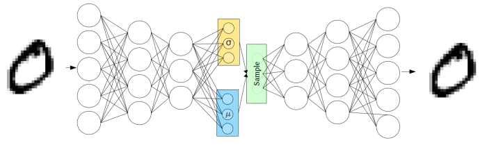
Where inputs \(x_i\) are encoded to vectors \(\mu\) and \(\log \sigma_i\), which parameterize \(q_\phi(z | x)\). Before decoding, we draw a sample \(z \sim q_\phi(z | x) = \mathcal{N}(\mu(x), \sigma(x)I)\) and evaluate its likelihood under the model with \(p_\theta(x | z)\). We compute the loss function \(\mathcal L(\theta, \phi ; x)\) and propagate its derivative with respect to \(\theta\) and \(\phi\), \(\nabla_\theta L\), \(\nabla_\phi L\), through the network during training.
Show Autograd VAE demo
Alternate derivation: Autoencoders
An autoencoder takes an input, encodes it into a vector, then decodes to produce something similar to the original data. Or: autoencoders reconstruct their own input using an encoder and a decoder.
Encoder: \(g(x) \rightarrow z \)
Decoder: \(f(z) \rightarrow \hat x\)
The encoder, \(g(x)\), takes in the input data (such as an image) and outputs a single value for each encoding dimension while the The decoder, \(f(z)\) takes this encoding and attempts to recreate the original input.
Our goal is to learn \(g, f\) from unlabeled data, and usually we specify f and g with neural networks, and minimize squared reconstruction error.

\(z\) is the code the model attempts to compress a representation of the input, \(x\), into. For deterministic autoencoders, it's important that this code is a bottleneck, i.e. that
as this forces the encoder to reduce the dimension, for example by learning how to ignore noise (otherwise, we would just learn the identify function). The big idea is that the code contains only the most important features of the input, such that we can reconstruct the input from the code reliably
Problems with Deterministic Autoencoders
There are two main problems with deterministic autoencoders.
Problem 1: Proximity in data space does not mean proximity in feature space
The embeddings (or codes) learned by the model are deterministic, i.e.
but proximity in feature space is not enforced for inputs in close proximity in data space, i.e.
If the space has regions where no data gets encoded to, and you sample/generate a variation from there, the decoder will simply generate an unrealistic output, because the decoder has no idea how to deal with that region of the latent space. During training, it never saw encoded vectors coming from that region of latent space.
Adding noise to autoencoders:
- Low-dim z. But what dimension?
- Can add noise to data before encoding, reconstruct original data. But how much noise?
- Can add noise to latents after encoding, reconstruct original data. But how much noise?
Variational Autoencoders (VAEs)
This stochastic generation means, that even for the same input, while the mean and standard deviations remain the same, the actual encoding will somewhat vary on every single pass simply due to sampling.
Why does a VAE solve the problems of a deterministic autoencoder?
The VAE generation model learns to reconstruct its inputs not only from the encoded points but also from the area around them. This allows the generation model to generate new data by sampling from an “area” instead of only being able to generate already seen data corresponding to the particular fixed encoded points.
What can we do with a latent variable model?
If a latent variable model has a compact prior and vector-valued \(z\)s, we can: - Sample new data to check the model - Encode (sample from the approximate posterior) of two datapoints, and interpolate between them in the latent space, then decode along the path - Learn a function to predict some property of the examples from the low-dimensional z space instead of directly from x. (Semi-supervised learning)
Tutorial
Consequences of using amortized inference
- Gradient updates of theta is like M-step . recognition network gives approximate E-step. Gradient updates of phi_r improves E-step
- Don’t need to re-optimize phi_i each time theta changes - much faster
- Recognition net won’t necessary give optimal phi_i
- Can have fast test-time inference (vision)
Semi-amortized inference:
There's no reason why we can't use a recognition network to initialize q, then take a few steps of SVI.
Alternate forms of the ELBO:
We also talked about two other alternative forms or "intuitions" of the ELBO:
The second of which (intuition 3) is the loss function we use for training VAEs. Notice now that the first term corresponds to the likelihood of our input under the distribution decoded from \(z\) and the second term the divergence of the approximate distribution posterior from the prior of the true distribution.
Note
The second terms acts a regularization, by enforcing the idea that our parameterization shouldn't move us too far from the prio distribution. Also note that this term as a simple, closed form if the posterior and prior are Gaussians.
Automatically choosing latent dimension
Standard autoencoders require choosing latent dimension What happens if a VAE has more than it needs? If q(z|x) is factorized, then KL term factorizes over dimensions, wants to make each q(z_i|x) look like p(z_i). If a dimension doesn’t help likelihood enough, it will ‘turn off’ and set q(z_i|x) = p(z_i), ignoring x. Then decoder can ignore too.